Graphs in Data Structures

Graphs

A graph in data structures G consists of two things:

1. A set v of elements called nodes (or points or vertices)
2. A set E of edges such that each edge e in E is identified with a unique (unordered) pair [u,v] of nodes in v, denoted by e=[u,v]sometimes we indicate the parts of a parts of a graph by writing G=(v,E).

Examples:

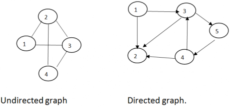  G=(V,E)                                                       G=(V,E) V={1, 2, 3, 4}                                    V={1, 2, 3, 4, 5} E={(1,2);(2,3);(2,4);(3,4);(1,3)}       E={(1,2) (1,3) (3,2) (3,5) (3,4) (4,2) (5, 4)} Suppose e=[u,v] then the nodes u and v are called the end points of e ,and u and v are said to be adjacent nodes or neighbors. An edge with an orientation is a directed edge while an edge with no orientation is an undirected edge. The undirected edges (i,j) and (j,i) are the same; the directed edge(i,j) is different from the directed edge(j,i). If all the edges in a graph are undirected, then the graph is undirected graph. The graphs of figure(a) and are undirected graphs. If all the edges are directed , then the graph is directed graph. The graph of figure(b) is a directed graph. Often an undirected graph is a simply called a graph and a directed graph is called a digraph.   In some applications of graphs and graphs we shall assign a weight or cost to each edge, when weights have been assigned to edges we use the terms weighted graph and weighted digraph. To refer to the resulting data object the term network refers to a weighted graph or digraph. Example:  

 

Representation of graphs and  Digraphs in data structures

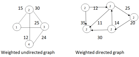
The most frequently used representation schemes for graphs and digraphs are adjacently based adjacency matrices and linked adjacency list.    

1. Adjacency Matrix:

The adjacency matrix of an n-vertex graph G=(V,E) is an nXn matrix A, each element of A is either zero or one .We shall assume that V={1, 2, 3, . . . . . n}.If G is a graph, then the elements of A are defined as follows.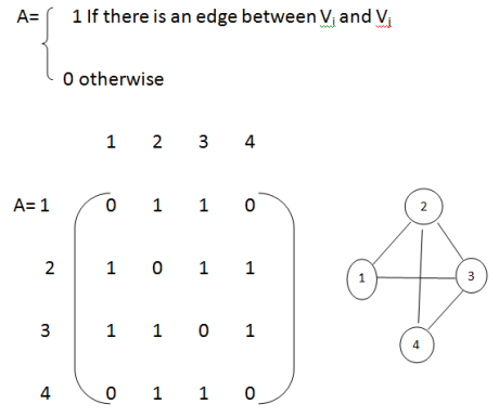    

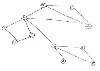
1. Linked –adjacency list:

In the case of linked adjacency lists, let G be a graph with m nodes.  The array representation of G in memory i.e., the representation of G by its adjacency matrix A has a number of major drawbacks. Consider the graph G in figure (a).The table shows each node in G followed by its adjacency list, which it  its list of adjacent nodes also called its successors or neighbours.Figure represents a schematic diagram of linked representation of G in memory specifically, the linked representation will contain two lists (or files), a node list NODE and edge list EDGE.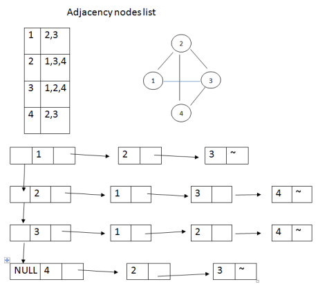      

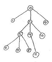
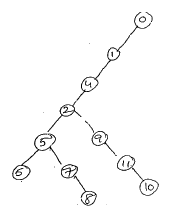
Traversing a Graph:

Many graph algorithms require one of systematically examine the nodes and edges of graph G. There are two standard ways that this is done one way is called a breadth first search and the other is called a depth- first search. The breadth – first search will use a queue as an auxiliary structure to hold nodes for future processing and analogously .The depth –first search will use a stack.

1. Breadth –first traversal : [B F S]

A data structure queue is used to place all waiting nodes. This queue is also convenient to keep the track of nodes that are already.  

Algorithm:

1. All nodes are initialized as ready states and initialise queue to empty.
2. Begin with any node, which is in ready state and put into queue. Mark the status of that node to waiting
3. While queue is not empty do begin.
4. Delete the first node k from queue and process it mark the status of that node.
5. Add all the adjacent nodes of k which are in ready state to the rear side of the queue and mark the status of these nodes to waiting.
6. If this graph still contains nodes which are in ready which are in ready state then go to step(2)
7.  

 

Dept-First search (DFS):

In the depth –first search traversal, we back track on a path once it reached the end of the path. We consider the data structure stack instead of a queue as in breadth first search.

Algorithm:

1. All nodes are initialized to ready state and initialize stack to empty.
2. Begin with any node which is in ready state and path into stack mark the status of that node to waiting.
3. While stack in not empty do begin.
4. Pop to node of stack and process it mark the status of that node to be visited.

5. Push at the adjacent nodes of k which are in ready state into stack and mark the stack of those nodes to waiting.
6. If the graph still contains nodes which are in ready state then go to step(2).
7.  

 

Example for BFS:

Adjacency nodes lists:

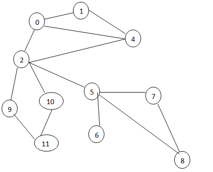
1	1,2,4
2	0,4
3	0,4,5,9,10
4	0,1,2
5	2,6,7,8
6	5
7	5,8
8	5,7
9	2,11
10	2,11
11	9,10

   

 After Traversing the BFS graph:

 

Example for DFS:

 

0	1,2,4
1	0,4
2	0,4,5,9,10
4	0,1,2
5	2,6,7,8
6	5
7	5,8
8	5,7
9	2,11
10	2,11

 

After traversing the DFS: